Analysis
Select a project in Jobs to reset the previous display and load only that project's structures, properties, spectra, and files. The job table uses the project name; the short internal identifier is retained only for unique storage.
Job and file controls
Depending on status, a job provides controls to open, stop, restart, or delete it. Deleting a project removes its managed result directory and should be used only after preserving any files needed elsewhere.
Project files lists the actual input and output files. Selecting a supported file updates the structure or data source. Optimization, IRC, NEB, dynamics, and other multi-frame results expose a frame or optimization-step control. Edit in Builder sends the selected structure back to Builder for a new calculation.
Results summary
The summary distinguishes the reference SCF energy from correlated or state-specific results. For DFT and HF jobs, the SCF energy is normally the principal electronic energy. For MRSF-TDDFT, correlated, EKT, and other methods, use the separately labeled state or method energies; an SCF reference energy is not an MRSF-TDDFT state energy.
Available summaries can include:
- total and state energies, excitation energies, and oscillator strengths;
- optimization convergence and step data;
- dipole and atomic population results;
- EKT ionization/electron-affinity roots and Dyson strengths;
- NMR shielding tensors and isotropic values; and
- vibrational frequencies and thermochemical quantities.
Structures and reaction paths
Optimization steps can be selected individually. The selected step updates the molecular structure, its recorded values, and state-resolved plots where those values were written for each step. Reaction-path calculations display relative energy against the path coordinate; selecting a point selects its structure.
Compare projects reports current-minus-reference energy, aligned Cartesian RMSD, dipole-magnitude change, and matched excited-state changes when the two projects contain the required data. It does not merge or rename either project.
Spectra
Studio shows only spectrum types supported by the selected project's output:
- Absorption uses S0-to-excited-state energies and oscillator strengths.
- Emission is offered for an excited-state structure with the corresponding downward transition data, not merely for a vertical excitation at S0 geometry.
- Excited-state absorption (ESA) uses transitions from the selected current excited state to higher states. For example, S1-to-S2 uses its own transition energy, not the absolute S2 energy.
- IR uses calculated frequencies and intensities.
- Photoelectron and inverse photoelectron spectra use EKT IP/EA roots and Dyson strengths.
Electronic transition energies are converted to wavelength with
lambda (nm) = 1239.841984 / Delta E (eV). Zero or non-positive transition
energies are excluded rather than producing an unbounded wavelength axis.
Choose Lorentzian, Gaussian, or pseudo-Voigt broadening, adjust the FWHM, and
export the sticks and curve as CSV.
Orbitals and volumetric maps
SCF molecular orbital lists orbitals from the normal SCF Molden output. Selecting an orbital generates its surface; no orbital is shown until one is selected. Reset map returns to the molecule.
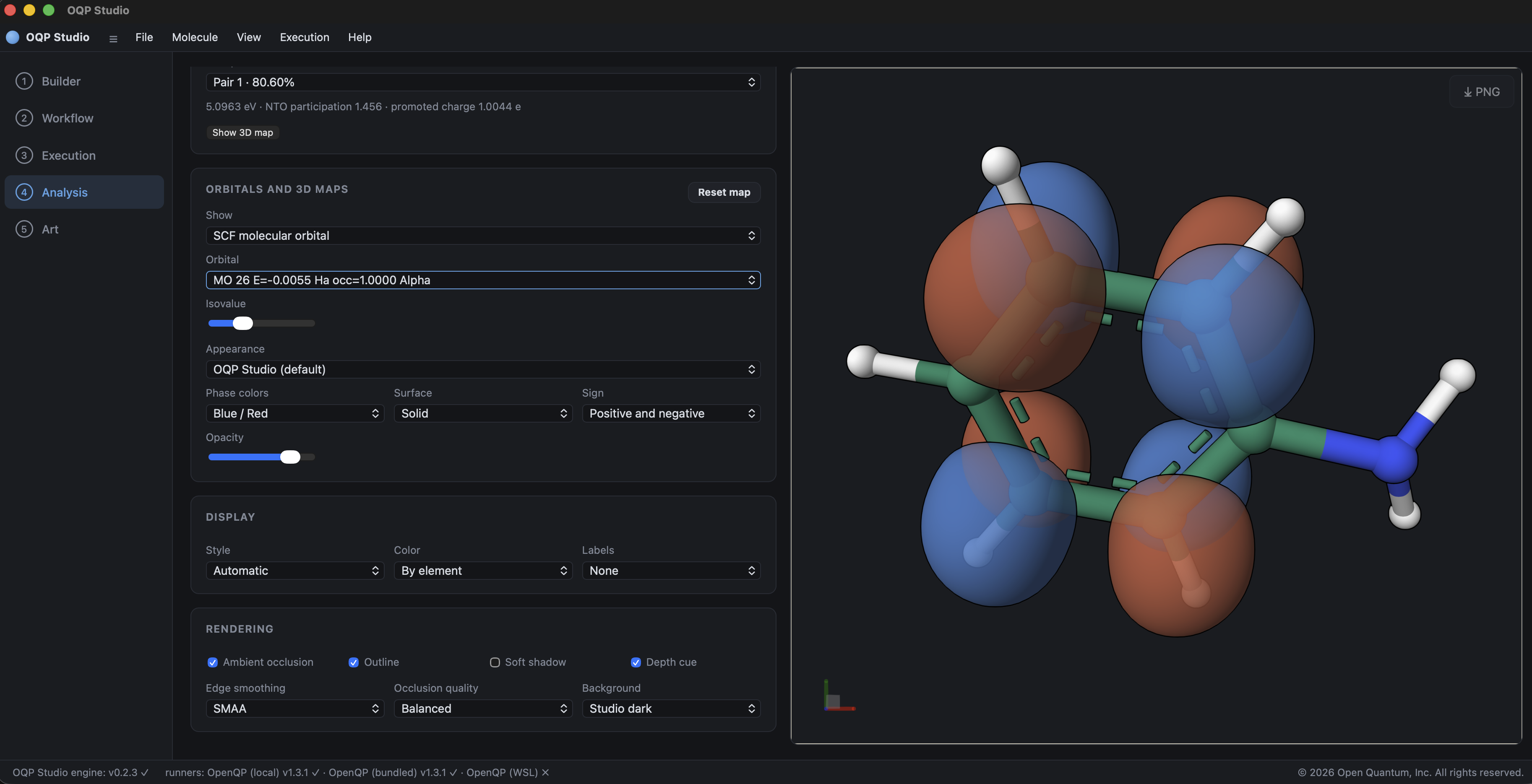
Analysis links the selected orbital and its energy and occupation to the three-dimensional positive and negative phases. The isovalue, color pair, surface style, sign, and opacity controls change the visualization without changing the calculated orbital.
For an IP/EA job with a Dyson Molden file, Dyson orbital appears as a
separate Show choice. Dyson orbitals are state specific and are labeled by IP
or EA root and source state where available. OpenQP's Dyson STRENGTH is shown
as strength; the corresponding occupation contribution is twice that value.
It is not mixed into the SCF orbital list.
Electron density, spin density, and electrostatic potential maps are generated when the orbital data needed for them are available. Existing cube files can be displayed directly. Two compatible grids can be summed or subtracted; Studio rejects grids whose dimensions, origin, axes, or atoms do not match instead of silently resampling them.
Excited-state maps and NTOs
When OpenQP exports the state-resolved transition density and matching Cartesian-basis orbital information, Excited-state analysis provides:
- NTO hole and particle pairs with singular-value weights;
- attachment and detachment densities;
- difference and transition densities; and
- target-state density.
Choose source and target states, then choose the map. If the required saved
transition density is absent, Studio reports that the analysis is unavailable;
it does not construct an NTO from excitation energies alone. A rerun may require
guess(save_mol=true) and an OpenQP build that exports the relevant
OQP::td_trans_density_mo result.
Normal modes
For a Hessian result, choose a value from Choose a normal mode. Selection alone displays the equilibrium molecule with optional displacement arrows. Play animates displacement continuously about the equilibrium structure; Pause stops at the current phase, and Reset restores equilibrium. Arrow visibility is independent of animation state. The amplitude control changes the visual displacement and does not alter the calculated normal mode.
Atomic properties
Atomic data can be displayed as labeled 3D maps, including Mulliken, Lowdin, and RESP charges and coupled NMR shielding when exported by OpenQP. The legend shows the numeric range. These atom-centered maps are distinct from volumetric cube surfaces.