Worked Examples
Each worked example is one small molecule, one complete .oqp input that you
can copy and run as it is, and the results that the run produces. The
coordinates are written inside the input, so no separate geometry file is
needed. Some examples need extra files, downloaded with them into the same
folder: the QM/MM examples read their structure and force
field from a PDB file and two OpenMM XML files, and the all-electron inputs of
the gold hydride example read an uncontracted basis set
from a JSON file, the NEB example reads its product structure
from an XYZ file, and the alanine QM/MM example reads a PDB
file. Run the input, then compare your numbers with the reference values on
the page.
openqp water-scf.oqp
Every input on these pages can also be downloaded from the link under its code block. With 2 to 8 CPU threads, most runs take between 2 seconds and 1 minute. These take longer:
| Example | Run time |
|---|---|
| HCN IRC, each direction | about 3.5 minutes |
| NH₃ NEB on the 150 × 974 DFT grid | about 7 minutes |
| Ethylene MECI search | about 3.5 minutes |
| NH₃ inversion NEB | about 7 minutes |
| Ethylene S1 minimum-energy path | about 4.5 minutes |
| Methanol ground-state MD | about 4.5 minutes |
| Formaldehyde QM/MM excited-state dynamics | about 5 minutes |
| Alanine-dipeptide QM/MM ground-state MD | about 6 minutes |
| Formaldehyde SOC-NAMD | about 2.5 minutes |
| Ethylene NAMD | about 9 minutes |
Benzene HF/cc-pVTZ with symmetry(enabled=false) |
about 1.5 minutes |
| Alanine-dipeptide QM/MM optimization | about 1 minute |
Each page states its run time.
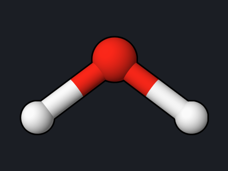
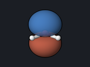 Water energy and orbitals
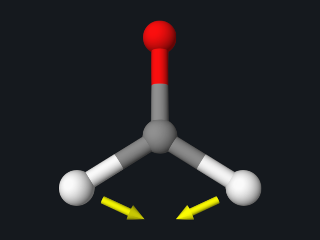 Geometry and vibrations
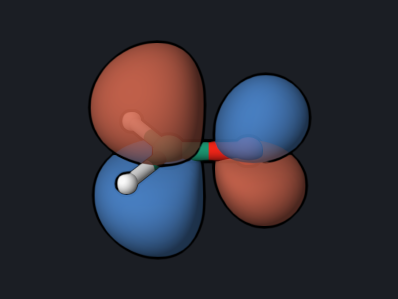 UV absorption (TDDFT)
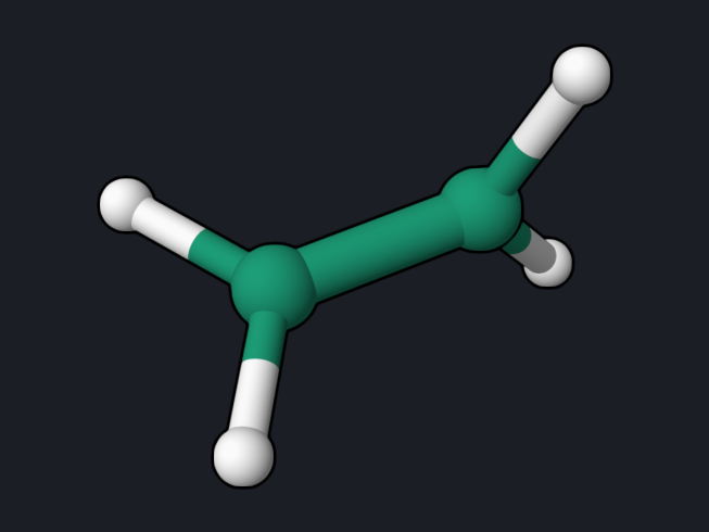 Twisted ethylene (MRSF-TDDFT)
S0, S1, and S2 along the C=C twist, where S0 becomes a diradical.
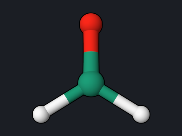 Spin-orbit coupling
Singlet-triplet coupling matrix elements in cm⁻¹ and El-Sayed's rule.
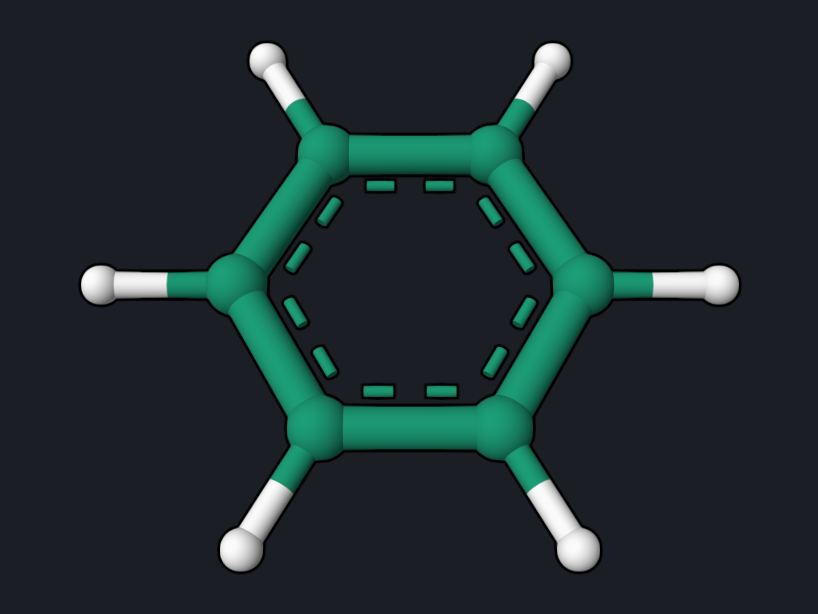 NMR chemical shifts
GIAO shieldings of benzene and TMS, converted to ¹H and ¹³C chemical shifts.
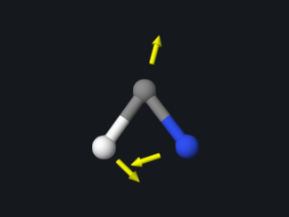 Transition state and barrier
 MP2 and CCSD(T) energies
Correlation energies of water at the MP2 and CCSD(T) levels.
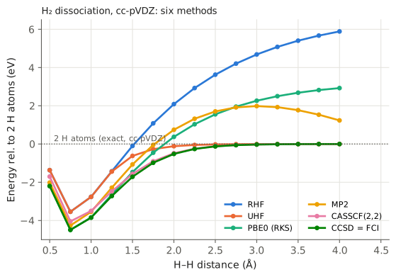 H₂ dissociation: six methods
RHF, UHF, PBE0, MP2, CASSCF, and CCSD along a breaking bond.
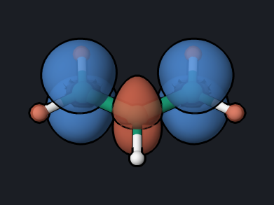 Allyl radical spin density
Open-shell UKS optimization, spin populations, and spin polarization.
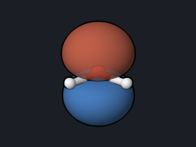 Ionization energies (MRSF-EKT)
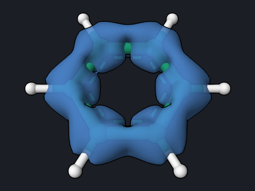 Ring current (ACID)
Current-density isosurface showing the aromatic ring current of benzene.
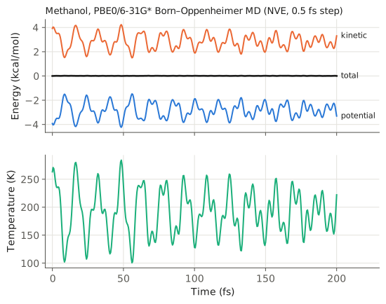 Ground-state MD
200 fs of Born–Oppenheimer dynamics and an energy-conservation check.
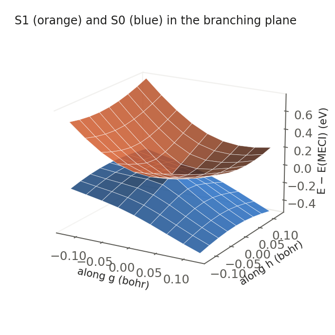 Conical intersection (MECI)
Locate the S0/S1 MECI of ethylene, its g and h vectors, and the cone.
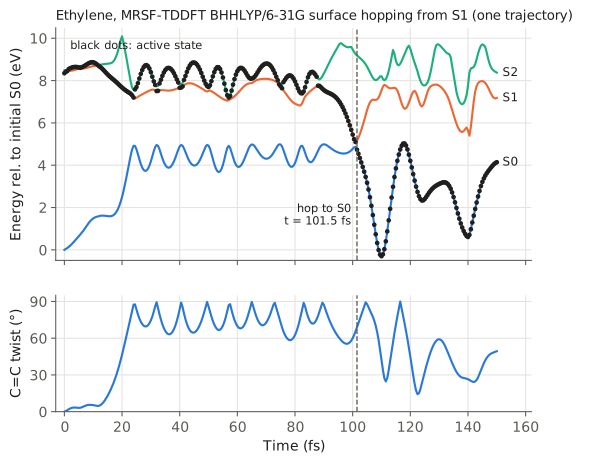 Nonadiabatic dynamics
Surface hopping from S1: twisting and return to S0 in 100 fs.
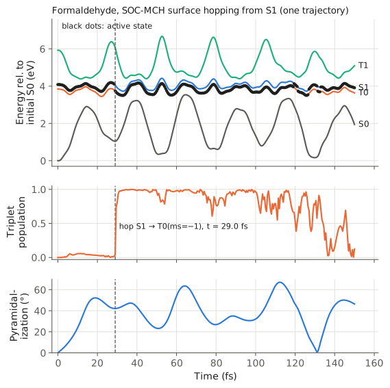 Intersystem crossing (SOC-NAMD)
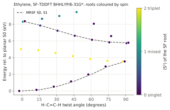 SF-TDDFT and spin contamination
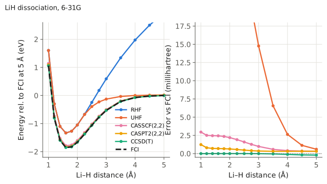 CASSCF and CASPT2 vs FCI
LiH dissociation with RHF, UHF, CASSCF, CASPT2, CCSD(T), and exact FCI.
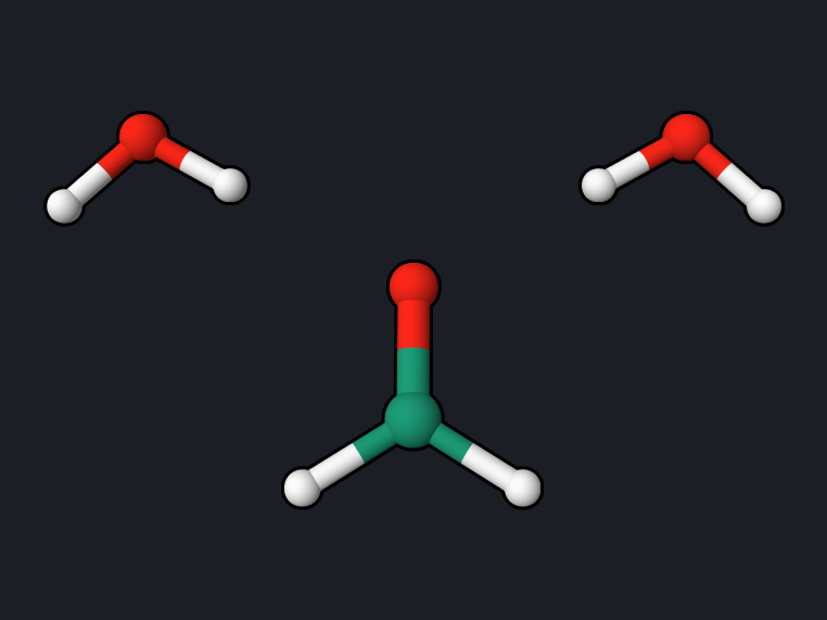 QM/MM solvent shift
n→π* shift of formaldehyde from two water molecules, QM/MM vs full QM.
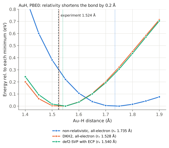 Relativity in gold hydride
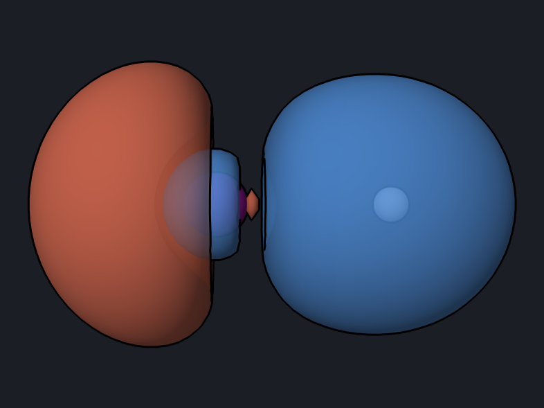 Effective core potentials
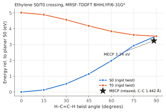 Singlet–triplet crossing (MECP)
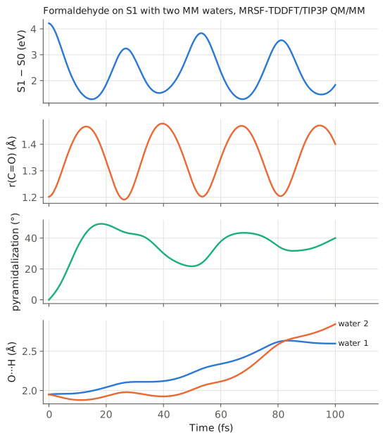 QM/MM excited-state dynamics
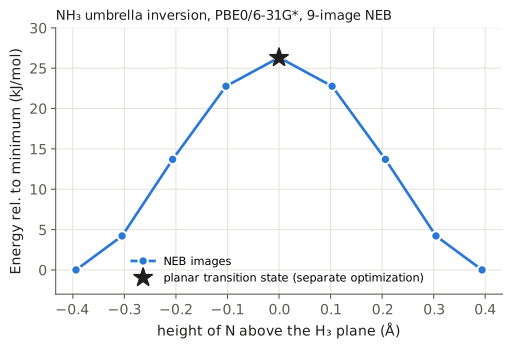 Reaction path by NEB
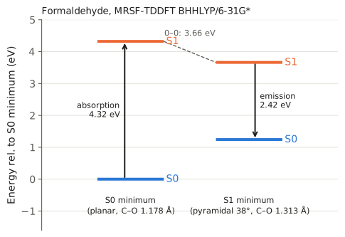 Excited-state optimization
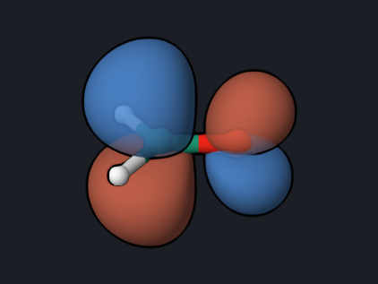 Python API and state analysis
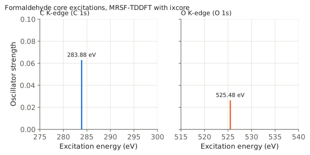 X-ray absorption
Carbon and oxygen K-edges of formaldehyde with MRSF-TDDFT ixcore.
UMRSF-TDDFT
MRSF-TDDFT with an unrestricted (UHF) triplet reference, compared with ROHF.
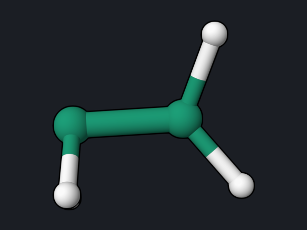 Coupling between geometries (NACME)
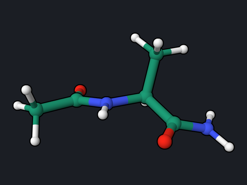 QM/MM across a covalent bond
Link-atom QM/MM optimization and dynamics of the alanine dipeptide.
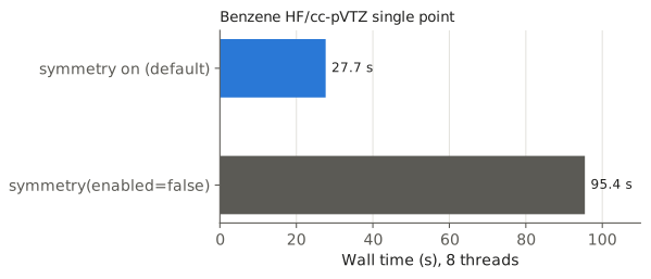 Molecular symmetry
Point-group detection, orbital labels, and a 3.4× faster SCF for benzene.
How the reference values were produced
All reference values on these pages come from running exactly the inputs shown,
with OpenQP 1.3.1 (GitHub main, commit f5361a2, 20 October 2026) on macOS
x86_64 with 2 to 8 OpenMP threads. The one exception is the
SOC-NAMD example: it needs the fix in
openqp#535 and was
run with GitHub main commit 958495f plus that fix (commit 20272ac5b).
The NEB example was rerun with commit 958495f plus the
frequency-projection fix in
openqp#538
(commit be1c9d2); no value on that page depends on that fix.
The absolute IR intensities on the
frequency page come from GitHub
main commit 0b75a06, which includes the IR unit fix
openqp#533,
as do the frequency tables of the HCN and
NH₃ transition states.
Molecule and orbital pictures are snapshots
of the OQP Studio 3D viewer, made from the output files of
the same runs.
On another computer, SCF energies normally agree with the reference values to about 10⁻⁶ hartree. Small differences in the last digits come from DFT integration grids, thread counts, and convergence thresholds. They are not errors.
Where an independent code was available, the reference values were also checked against PySCF 2.13 at the same geometry and basis set. Each page states which values were checked.
Reading an OpenQP run
Every run writes these files beside the input:
| File | Contents |
|---|---|
<name>.log |
The full text output, including SCF iterations, orbital energies, and all requested properties. Each page quotes the relevant part. |
<name>_scf_*.molden |
Molecular orbitals in Molden format. Open it in OQP Studio Analysis, OpenqpView, Molden, or Avogadro to display orbitals. |
<name>.hess.json, <name>.freq.molden |
Written by Hessian runs: frequencies, normal modes, and thermochemistry data. Open the .freq.molden file to animate the vibrations. |
opt.xyz, opt_status.txt |
Written by geometry optimizations and transition-state searches: the final geometry and a table of the optimization steps. |
The end of every log has an ENERGIES AND STATES block, which is the quickest
place to read the final energies:
   PyOQP LOG | ENERGIES AND STATES
   PyOQP: Final Energy
   ========================================================================
   PyOQP Energy unit:                 Hartree
   PyOQP electronic energies
   PyOQP state 0                            -76.3256993935
For the full input syntax, see .oqp Input. For larger
template decks, see the repository examples.