H₂ Dissociation: Six Methods Compared¶

Pulling apart H₂ is the simplest test of how a method treats a breaking bond. Near equilibrium almost every method works. At long distance the two electrons must end up one on each hydrogen, and only methods that can describe that situation reach the correct limit of two hydrogen atoms. This example runs six OpenQP methods along the same curve.

H2 dissociation curves

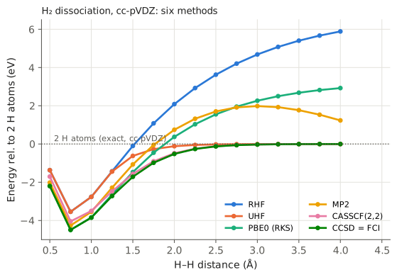
The zero of energy is two separate hydrogen atoms in the same basis set. Every point on the curves above is a separate OpenQP run.

Copy and run¶

The six inputs below differ only in the first line. Each is shown at r(H–H) = 2.0 Å:

h2-ccsd.oqp

ccsd/cc-pvdz
geom="""
H      0.000000     0.000000     0.000000
H      0.000000     0.000000     2.000000
"""

Method	First line	Download
RHF	`rhf/cc-pvdz`	h2-rhf.oqp
UHF	`uhf/cc-pvdz scf(stability=true)`	h2-uhf.oqp
PBE0	`dft/pbe0/cc-pvdz`	h2-pbe0.oqp
MP2	`mp2/cc-pvdz`	h2-mp2.oqp
CASSCF(2,2)	`casscf/cc-pvdz cas(active_electrons=2,active_orbitals=2)`	h2-casscf.oqp
CCSD	`ccsd/cc-pvdz`	h2-ccsd.oqp

Each run takes 1–3 seconds. To produce the whole curve, this script writes one input per method and distance:

methods = {
    "rhf": "rhf/cc-pvdz",
    "uhf": "uhf/cc-pvdz scf(stability=true)",
    "pbe0": "dft/pbe0/cc-pvdz",
    "mp2": "mp2/cc-pvdz",
    "casscf": "casscf/cc-pvdz cas(active_electrons=2,active_orbitals=2)",
    "ccsd": "ccsd/cc-pvdz",
}
for i in range(15):
    r = 0.5 + 0.25 * i
    for name, route in methods.items():
        with open(f"h2_{name}_{r:.2f}.oqp", "w") as f:
            f.write(f'{route}\ngeom="""\nH 0.0 0.0 0.0\nH 0.0 0.0 {r:.6f}\n"""\n')

for f in h2_*.oqp; do openqp "$f"; done

Read each final energy from the PyOQP state 0 line of the ENERGIES AND STATES block.

What you get¶

Total energies in hartree:

Method	r = 0.75 Å	r = 4.00 Å	Behaviour at long distance
RHF	−1.12874	−0.78220	5.9 eV too high: both electrons forced into one orbital
UHF	−1.12874	−0.99857	correct limit, after the spin symmetry breaks
PBE0	−1.16353	−0.89104	2.9 eV too high
MP2	−1.15521	−0.95319	the curve turns over and falls again
CASSCF(2,2)	−1.14721	−0.99860	correct limit
CCSD	−1.16359	−0.99861	correct limit; exact for two electrons

Reading the result¶

CCSD is exact here. For a two-electron system CCSD equals full configuration interaction, so its curve is the reference for the others in this basis set. At 0.75 Å it lies 4.49 eV below the two atoms.
RHF puts both electrons in the same spatial orbital at every distance, so half of the wavefunction at long distance is the ionic H⁺H⁻ configuration. The energy rises far above two atoms.
UHF gives the same answer as RHF up to 1.0 Å; by 1.25 Å it is lower. Beyond this point, a lower solution exists where the α and β electrons localize on different atoms. scf(stability=true) tells OpenQP to test the converged RHF-like solution and follow the instability to this lower solution; without it, the UHF run stays on the RHF curve.
MP2 is built on the RHF reference. Its correction grows without bound as the HOMO–LUMO gap closes, so the curve turns over after 2.75 Å.
CASSCF(2,2) includes both the bonding and antibonding configurations and dissociates correctly, but misses the remaining (dynamic) correlation, so its well is shallower than CCSD near equilibrium.
PBE0 with a closed-shell (restricted) reference has the same problem as RHF, softened by the functional.

Try next¶

Repeat the scan with cc-pvtz and compare the CCSD well depth with the experimental dissociation energy, 4.75 eV.
Use the same script with a different molecule, for example LiH, where the frozen core and active-space choices start to matter.